DDPM

Denoising Diffusion Probabilistic Models

Takeaways

• A diffusion probabilistic model is a parameterized Markov chain trained using variational inference to produce samples matching the data after finite time.
• Transitions of this chain are learned to reverse a diffusion process, which is a Markov chain that gradually adds noise to the data in the opposite direction of sampling until signal is destroyed.
• When the diffusion rates \(\beta_t\) are small, it is sufficient to set the sampling chain transitions to conditional Gaussians too, allowing for a particularly simple neural network parameterization.
• DDPM shows that diffusion models are capable of generating high quality samples.

Introduction

Let \(X_0\sim q(x_0)\) be the data distribution. The forward process (diffusion process) \(q(x_{1:T}\vert x_0)\) of diffusion models is a Markov chain that generates latent variables \(X_1,\dots,X_T\) by gradually adding Gaussian noise to the data \(X_0\) according to a variance schedule \(\beta_1,\dots,\beta_T\) where

\[q(x_{1:T}|x_0):=\prod_{t=1}^T q(x_t|x_{t-1}),\quad q(x_t|x_{t-1}):=\mathcal{N}(x_t;\sqrt{1-\beta_t}x_{t-1},\beta_t I)\]

choices of \(\beta_t\)

• learned by reparameterization
• held constant as hyperparameters

The diffusion models aim to learn a generative distribution \(p_\theta\) to describe the same trajectory, but in reverse,

\[p_\theta(x_{0:T}):=p(x_T)\prod_{t=1}^T p_\theta(x_{t-1}|x_t),\quad p(x_T)=\mathcal{N}(x_t;0,I)\]

The reverse processes have the same functional form (Gaussian) when \(\beta_t\) are small (the time reversibility of SDE). Therefore, diffusion models learn Gaussian distribution in the reverse Markov chain:

\[p_\theta(x_{t-1}|x_t):=\mathcal{N}(x_{t-1};\mu_\theta(x_t, t), \Sigma_\theta(x_t, t))\]

Training is performed by optimizing the usual variational bound on negative log likelihood (see Appendix for details):

\[\mathbb{E}_q[-\log p_\theta(X_0)] \le \mathbb{E}_q\left[-\log p(X_T)-\sum_{t=1}^T\log\frac{p_\theta(X_{t-1}|X_t)}{q(X_t|X_{t-1})} \right] =:L\\\]

The loss \(L\) can be rewritten as

\[L =\mathbb{E}_q\left[\underbrace{D_\text{KL}(q(x_T|X_0)||p(x_T))}_{L_T}+\sum_{t=2}^T \underbrace{D_\text{KL}(q(x_{t-1}|X_t,X_0)||p_\theta(x_{t-1}|X_t))}_{L_{t-1}} \underbrace{-\log p_\theta(X_0|X_1)}_{L_0} \right]\]

When conditioned on \(X_0\), both \(X_t\) and \(X_{t-1}\) are Gaussian (see Appendix):

\[q(x_t|x_0)=\mathcal{N}(x_t;\sqrt{\overline{\alpha}_t}x_0,(1-\overline{\alpha}_t)I),\quad q(x_{t-1}|x_0)=\mathcal{N}(x_{t-1};\sqrt{\overline{\alpha}_{t-1}}x_0,(1-\overline{\alpha}_{t-1})I),\]

where \(\alpha_t:=1-\beta_t\) and \(\overline{\alpha}_t:=\prod_{s=1}^t\alpha_s\). According to the forward model, we have the following reparameterization: \(X_t=\sqrt{\alpha_t}X_{t-1}+\sqrt{1-\alpha_t}\epsilon_t\), with \(\epsilon_t\in\mathcal{N}(0,I)\) and therefore, \(\text{Cov}(X_t,X_{t-1})=\sqrt{\alpha_t}\text{Var}(X_{t-1})\) and the posterior conditioned on \(X_0\) is

\[q(x_{t-1}|x_t,x_0)=\mathcal{N}(x_{t-1};\tilde{\mu}_t(x_t,x_0),\tilde{\beta}_tI),\]

where

\[\tilde{\mu}_t(x_t,x_0):=\frac{\sqrt{\overline\alpha_{t-1}}\beta_t}{1-\overline\alpha_t}x_0+\frac{\sqrt{\alpha_t}(1-\overline{\alpha}_{t-1})}{1-\overline{\alpha}_t}x_t,\quad \tilde{\beta}_t:=\frac{1-\overline\alpha_{t-1}}{1-\overline\alpha_{t}}\beta_t\]

DDPM

Forward process and \(L_T\)

Fix \(\beta_t\) to constants, the approximate posterior \(q\) has no learnable parameters, and \(L_T\) is a constant.

Reverse process and \(L_{1:T-1}\)

\[p_\theta(x_{t-1}|x_t):=\mathcal{N}(x_{t-1};\mu_\theta(x_t, t), \Sigma_\theta(x_t, t))\]

Variances

Set \(\Sigma_\theta(x_t,t)=\sigma_t^2I\) to untrained time-dependent constants. Experimentally, the following two choices of \(\sigma_t^2\) have similar results.

• Choice 1: \(\sigma_t^2=\beta_t\). This optimial for \(X_0\sim\mathcal{N}(0,I)\). (see Appendix)

• Choice 2: \(\sigma_t^2=\frac{1-\overline\alpha_{t-1}}{1-\overline\alpha_t}\beta_t\). This is optimal for \(X_0\) deterministically set to one point. (see Appendix)

Means

We rewrite \(L_{t-1}\) as follows. (see Appendix)

\[L_{t-1}=\mathbb{E}_q\left[ \frac{1}{2\sigma_t^2}\| \tilde\mu_t(X_t, X_0) -\mu_\theta(X_t,t)\|_2^2 \right]+C\]

where \(C\) is a constant that does not depend on \(\theta\). Since \(X_t=\sqrt{\overline\alpha_t}X_0+\sqrt{1-\overline\alpha_t}\epsilon\) for \(\epsilon\sim\mathcal{N}(0,I)\).

\[\begin{aligned} L_{t-1}-C&=\mathbb{E}_{X_0,\epsilon}\left[ \frac{1}{2\sigma_t^2}\left\| \tilde\mu_t\left(X_t, \frac{1}{\sqrt{\overline\alpha_t}}(X_t-\sqrt{1-\overline\alpha_t}\epsilon)\right) -\mu_\theta(X_t,t)\right\|_2^2 \right]\\ &=\mathbb{E}_{X_0,\epsilon}\left[ \frac{1}{2\sigma_t^2}\left\| \frac{1}{\sqrt{\alpha_t}} \left(X_t-\frac{\beta_t}{\sqrt{1-\overline\alpha_t}}\epsilon\right)-\mu_\theta(X_t,t)\right\|_2^2 \right] \end{aligned}\]

Since \(X_t\) is available as input to the model, we may choose the parameterization

\[\mu_\theta(X_t, t):= \frac{1}{\sqrt{\alpha_t}} \left(X_t-\frac{\beta_t}{\sqrt{1-\overline\alpha_t}}\epsilon_\theta(X_t, t)\right)\]

To sample \(X_{t-1}\sim p_\theta(x_{t-1}\vert x_t)\) is to compute

\[X_{t-1}=\frac{1}{\sqrt{\alpha_t}} \left(X_t-\frac{\beta_t}{\sqrt{1-\overline\alpha_t}}\epsilon_\theta(X_t, t)\right)+\sigma_t z,\]

where \(z\sim\mathcal{N}(0,1)\). With the parameterization of \(\mu_\theta\), the loss simplifies to

\[\mathbb{E}_{X_0,\epsilon}\left[ \frac{\beta_t^2}{2\sigma_t^2\alpha_t(1-\overline\alpha_t)}||\epsilon-\epsilon_\theta(\sqrt{\overline\alpha_t}X_0+\sqrt{1-\overline\alpha_t}\epsilon,t) ||_2^2 \right]\]

Data Scaling, Reverse Process Decoder, and \(L_0\)

Assume that image data consists of integers in \(\{0,1,\dots,255\}\) and scale them ilnearly to \([-1,1]\). This ensures that the neural network reverse process operates on consistently scaled inputs starting from the standard normal prior \(p(x_T)\). Set the last term of the reverse process as follows:

\[p_\theta(x_0|x_1)=\prod_{i=1}^D\int_{\delta_-(x_0^i)}^{\delta_+(x_0^i)}\mathcal{N}(x;\mu_\theta^i(x_1,1),\sigma_1^2)dx,\] \[\delta_+(x)=\left\{ \begin{aligned} &\infty &\text{if } x=1 \\ &x+\frac{1}{255} &\text{if } x<1 \end{aligned} \right., \qquad \delta_-(x)=\left\{ \begin{aligned} &-\infty &\text{if } x=-1 \\ &x-\frac{1}{255} &\text{if } x>-1 \end{aligned} \right.,\]

where \(D\) is the data dimensionality and the \(i\) superscript indicates extraction of one coordinate. Similar to the discretized continuous distributions used in VAE decoders and autoregressive models, the choice here ensures that the variational bound is a lossless codelength of discrete data, without the need of adding noise to the data or incorporating the Jacobian of the scaling operation into the log likelihood.

At the end of sampling, \(\mu_\theta(X_1, 1)\) is outputed without adding noise.

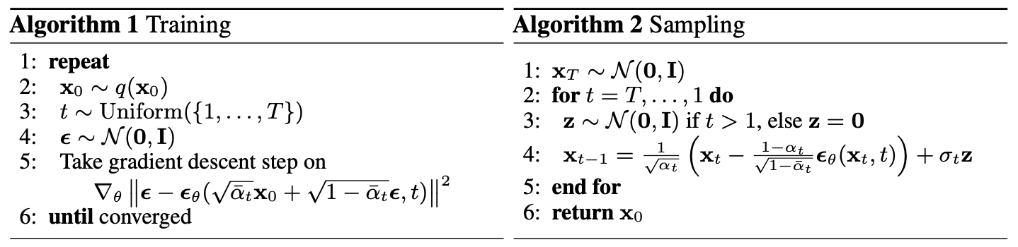
Training and Sampling

It is beneficial to sample quality (and simpler to implement) to train on the following variant of the variational bound:

\[L_\text{simple}(\theta):=\mathbb{E}_{t,X_0,\epsilon}\left[ \| \epsilon-\epsilon_\theta(\sqrt{\overline\alpha_t}X_0+\sqrt{1-\overline\alpha_t}\epsilon,t) \|_2^2 \right],\]

where \(t\) is uniform between \(1\) and \(T\).

• The \(t=1\) case corresponds to \(L_0\)
• The \(t>1\) cases correspond to an unweighted version of \(L_{t-1}\).
• The \(L_T\) term does not appear because the forward process variances \(\beta_t\) are fixed.

Since the simplified objective discards the weighting, it is a weighted variational bound that emphasizes different aspects of reconstruction compared to the standard variational bound. The diffusion process setup in the experiments causes the simplified objective to down-weight loss terms corresponding to small \(t\). These terms train the network to denoise data with very small amounts of noise, so it is beneficial to down-weight them so that the network can focus on more difficult denoising tasks at larger \(t\) terms.

The overall training and sampling algorithms are as follows.

Experiments

Hyperparameters

\(T\)	\(\beta_1\)	\(\beta_T\)	\(\beta\) intepolation
1000	\(10^{-4}\)	0.02	Linear

• Use a U-Net backbone with group normalization.
• Parameters are shared across time, which is specified to the network using the Transformer sinusoidal position embedding
• Use self-attention at the \(16 \times 16\) feature map resolution.

Sample Quality

• The unconditional DDPM achieves better sample quality than most models in the literature, including class conditional models.
• Training DDPMs on the true variational bound yields better codelengths (i.e., the negative log likelihoods) than training on the simplified objective, as expected, but the latter yields the best sample quality.

Reverse Process Parameterization and Training Objective Ablation

1. The baseline option of predicting \(\tilde\mu\) works well only when trained on the true variational bound instead of unweighted mean squared error.
2. Learning reverse process variances (by incorporating a parameterized diagonal \(\Sigma_\theta\) into the variational bound) leads to unstable training and poorer sample quality compared to fixed variances.
3. Predicting \(\epsilon\) performs approximately as well as predicting \(\tilde\mu\) when trained on the variational bound with fixed variances, but much better when trained with the simplified objective.

Progressive Coding

The lossless codelengths of DDPMs are better than the large estimates reported for energy-based models and score matching using annealed importance sampling, they are not competitive with other types of likelihood-based generative models.

DDPMs have an inductive bias that makes them excellent lossy compressors.

Progressive Lossy Compression

The distortion decreases steeply in the low-rate region of the rate-distortion plot, indicating that the majority of the bits are indeed allocated to imperceptible distortions

Progressive Generation

Experiment: Run a progressive unconditional generation process given by progressive decompression from random bits, i.e., predicting the result of the reverse process, \(\hat{X}_0=(X_t-\sqrt{1-\overline\alpha_t}\epsilon_\theta(X_t, t))/\sqrt{\overline\alpha_t}\), while sampling from the reverse process.

Result: Large-scale image features appear first and details appear last

Experiment: Stochastic prediction by sampling images from \(p_\theta(x_0\vert x_t)\) for different time step

Results: When \(t\) is small, all but fine details are preserved, and when \(t\) is large, only large-scale features are preserved. Perhaps these are hints of conceptual compression.

Connection to Autoregressive Decoding

The variational bound \(L\) can be rewritten as (see Appendix):

\[L=D_\text{KL}(q(x_T)||p(x_T)) + \mathbb{E}_q\left[\sum_{t=1}^TD_\text{KL}(q(x_{t-1}|X_t)||p_\theta(x_{t-1}|X_t))\right] + H(X_0)\]

An autoregressive model can be considered as a special diffusion model:

1. Set the diffusion process length \(T\) to the dimensionality of the data.
2. Define the forward process so that \(q(x_t\vert x_0)\) places all probability mass on \(x_0\) with the first \(t\) coordinates masked out (i.e., \(q(x_t\vert x_{t-1})\) masks out the \(t\)-th coordinate).
3. Set \(p(x_t)=q(x_t)\) to place all mass on a blank image, and therefore \(D_\text{KL}(q(x_T)\|p(x_T))=0\)
4. Take \(p_\theta(x_{t-1}\vert x_t)\) to be a fully expressive conditional distribution.
5. With these choices, minimizing \(D_\text{KL}(q(x_{t-1}\vert x_t)\|p_\theta(x_{t-1}\vert x_t))\) trains \(p_\theta\) to copy coordinates \(t+1,\dots,T\) unchanged and to predict the \(t\)-th coordinate given \(t+1,\dots,T\)

Insights:

• Interpret the Gaussian DM as a kind of autoregressive model with a generalized bit ordering that cannot be expressed by reordering data coordinates.

• Prior work has shown that such reorderings introduce inductive biases that have an impact on sample quality.

• Gaussian diffusion might serve a similar purpose, perhaps to greater effect since Gaussian noise might be more natural to add to images compared to masking noise. Gaussian diffusion length is not restricted to equal the data dimension: Gaussian diffusions can be made shorter for fast sampling or longer for model expressiveness.

Interpolation

Interpolate images in the latent space

1. Given two images from the data distribution \(X_0,X_0'\sim q(x_0)\).
2. Use \(q\) as a stochastic encoder to encoder \(X_0\) and \(X_0'\) into \(X_t\) and \(X_t'\) respectively, where \(X_t,X_t'\sim q(x_t\vert x_0)\).
3. Linearly interpolate in the latent space: \(\bar{X}_t=(1-\lambda)X_t+\lambda X_t'\).
4. Decode \(\bar{X}_t\) into the image space by the reverse process, \(\bar{X}_0\sim p(x_0\vert\bar{x}_t)\)

Results: The reverse process produces high-quality reconstructions and plausible interpolations that smoothly vary attributes such as pose, skin tone, hairstyle, expression, and background, but not eyewear. Larger \(t\) results in coarser and more varied interpolations.

Appendix

Variational Bound on Negative log Likelihood

\[\begin{aligned} \mathbb{E}_q[-\log p_\theta(X_0)] &=\int -q(x_0)\log p_\theta(x_0) d x_0 \\ & = \int -q(x_0)\log\left[\int\frac{p_\theta(x_{0:T})}{q(x_{1:T}|x_0)}q(x_{1:T}|x_0) d x_{1:T} \right]d x_0 \\ &\le \int -q(x_0)\int\log\left[\frac{p_\theta(x_{0:T})}{q(x_{1:T}|x_0)}\right]q(x_{1:T}|x_0) d x_{1:T} d x_0 \\ & = \int -q(x_{0:T})\log\frac{p_\theta(x_{0:T})}{q(x_{1:T}|x_0)} dx_{0:T} \\ & = \mathbb{E}_q \left[-\log\frac{p_\theta(X_{0:T})}{q(X_{1:T}|X_0)}\right] \\ & = \mathbb{E}_q \left[-\log\frac{p(X_T)\prod_{t=1}^T p_\theta(X_{t-1}|X_t)}{\prod_{t=1}^Tq(X_t|X_{t-1})}\right] \\ & = \mathbb{E}_q\left[-\log p(X_T)-\sum_{t=1}^T\log\frac{p_\theta(X_{t-1}|X_t)}{q(X_t|X_{t-1})} \right] =:L\\ \end{aligned}\]

To derive the objective for DDPM, \(L\) can be rewritten as

\[\begin{aligned} L & = \mathbb{E}_q\left[-\log p(X_T)-\sum_{t=1}^T\log\frac{p_\theta(X_{t-1}|X_t)}{q(X_t|X_{t-1})} \right]\\ & = \mathbb{E}_q\left[-\log p(X_T)-\sum_{t=2}^T\log\frac{p_\theta(X_{t-1}|X_t)}{q(X_t|X_{t-1})} - \log\frac{p_\theta(X_0|X_1)}{q(X_1|X_0)} \right] \\ & = \mathbb{E}_q\left[-\log p(X_T)-\sum_{t=2}^T\log\frac{p_\theta(X_{t-1}|X_t)}{q(X_t|X_{t-1}, X_0)} - \log\frac{p_\theta(X_0|X_1)}{q(X_1|X_0)} \right] \\ & = \mathbb{E}_q\left[-\log p(X_T)-\sum_{t=2}^T\log\frac{p_\theta(X_{t-1}|X_t)q(X_{t-1}|X_0)}{q(X_{t-1}|X_{t}, X_0)q(X_t|X_0)} - \log\frac{p_\theta(X_0|X_1)}{q(X_1|X_0)} \right] \\ & = \mathbb{E}_q\left[-\log \frac{p(X_T)}{q(X_T|X_0)}-\sum_{t=2}^T\log\frac{p_\theta(X_{t-1}|X_t)}{q(X_{t-1}|X_{t}, X_0)} - \log p_\theta(X_0|X_1)\right] \\ & = \mathbb{E}_q\left[\underbrace{D_\text{KL}(q(x_T|X_0)||p(x_T))}_{L_T}+\sum_{t=2}^T \underbrace{D_\text{KL}(q(x_{t-1}|X_t,X_0)||p_\theta(x_{t-1}|X_t))}_{L_{t-1}} \underbrace{-\log p_\theta(X_0|X_1)}_{L_0} \right] \end{aligned}\]

Here is another way to rewrite \(L\) which is helpful for analysis.

\[\begin{aligned} L & = \mathbb{E}_q\left[-\log p(X_T)-\sum_{t=1}^T\log\frac{p_\theta(X_{t-1}|X_t)}{q(X_t|X_{t-1})} \right]\\ &=\mathbb{E}_q\left[-\log p(X_T)-\sum_{t=1}^T\log\frac{p_\theta(X_{t-1}|X_t)}{q(X_{t-1}|X_{t})}\frac{q(X_{t-1})}{q(X_t)} \right]\\ &=\mathbb{E}_q\left[-\log \frac{p(X_T)}{q(X_T)}-\sum_{t=1}^T\log\frac{p_\theta(X_{t-1}|X_t)}{q(X_{t-1}|X_{t})}-\log q(X_0) \right]\\ &=D_\text{KL}(q(x_T)||p(x_T)) + \mathbb{E}_q\left[\sum_{t=1}^TD_\text{KL}(q(x_{t-1}|X_t)||p_\theta(x_{t-1}|X_t))\right] + H(X_0) \end{aligned}\]

Close Form of Forward Process

A notable property of the forward process is that it admits sampling \(X_t\) at an arbitrary timestep \(t\) in closed form: using the notation \(\alpha_t:=1-\beta_t\) and \(\overline{\alpha}_t:=\prod_{s=1}^t\alpha_s\), we have

\[q(x_t|x_0)=\mathcal{N}(x_t;\sqrt{\overline{\alpha}_t}x_0,(1-\overline{\alpha}_t)I)\]

Proof:

Let \(\epsilon_1,\dots,\epsilon_n\) be noise sampled iid from \(\mathcal{N}(0, I)\).

\[\begin{aligned} X_t&=\sqrt{\alpha_t}X_{t-1}+\sqrt{1-\alpha_t}\epsilon_t \\ &= \sqrt{\alpha_t}(\sqrt{\alpha_{t-1}}X_{t-2}+\sqrt{1-\alpha_{t-1}}\epsilon_{t-1})+\sqrt{1-\alpha_t}\epsilon_t \\ &=\dots \\ &=\sqrt{\alpha_t\cdots\alpha_1}X_0+\sqrt{\alpha_t\cdots\alpha_2}\sqrt{1-\alpha_1}\epsilon_1+\cdots+\sqrt{\alpha_t}\sqrt{(1-\alpha_{t-1})}\epsilon_{t-1}+\sqrt{1-\alpha_t}\epsilon_t \\ &=\sqrt{\overline{\alpha}_t}X_0+\sqrt{1-\overline\alpha_t}\overline\epsilon_t, \end{aligned}\]

where \(\overline\epsilon_t\sim\mathcal{N}(0, I)\). To obtain the last equality, we use the fact that

\[\begin{aligned} (\sqrt{\alpha_t\cdots\alpha_1})^2+(\sqrt{\alpha_t\cdots\alpha_2}\sqrt{1-\alpha_1})^2+\cdots+(\sqrt{\alpha_t}\sqrt{(1-\alpha_{t-1})})^2+(\sqrt{1-\alpha_t})^2&=1\\ (\sqrt{\alpha_t\cdots\alpha_2}\sqrt{1-\alpha_1})^2+\cdots+(\sqrt{\alpha_t}\sqrt{(1-\alpha_{t-1})})^2+(\sqrt{1-\alpha_t})^2&=1-\overline\alpha_t \end{aligned}\]

KL Divergence between Two Gaussian Distributions

Let \(p:=\mathcal{N}(\mu_p,\Sigma_p)\) and \(q:=\mathcal{N}(\mu_q,\Sigma_q)\) be two \(d\)-dimensional Gaussian distributions.

\[\begin{aligned} D_\text{KL}(p||q)&=\mathbb{E}_p\left[\log(p)-\log(q)\right] \\ &=\mathbb{E}_p\left[\frac{1}{2}\log\frac{|\Sigma_q|}{|\Sigma_p|}-\frac{1}{2}(X-\mu_p)^T\Sigma_p^{-1}(X-\mu_p)+\frac{1}{2}(X-\mu_q)^T\Sigma_q^{-1}(X-\mu_q)\right] \\ &=\frac{1}{2}\log\frac{|\Sigma_q|}{|\Sigma_p|}-\frac{1}{2}\mathbb{E}_p\left[(X-\mu_p)^T\Sigma_p^{-1}(X-\mu_p)\right]+\frac{1}{2}\mathbb{E}_p\left[(X-\mu_q)^T\Sigma_q^{-1}(X-\mu_q)\right] \end{aligned}\]

The second term is

\[\begin{aligned} \mathbb{E}_p\left[(X-\mu_p)^T\Sigma_p^{-1}(X-\mu_p)\right]&=\mathbb{E}_p\left[tr\{(X-\mu_p)^T\Sigma_p^{-1}(X-\mu_p)\}\right] \\ &=\mathbb{E}_p\left[tr\{(X-\mu_p)(X-\mu_p)^T\Sigma_p^{-1}\}\right] \\ &=tr\{\mathbb{E}_p\left[(X-\mu_p)(X-\mu_p)^T\Sigma_p^{-1}\right]\} \\ &=tr\{\mathbb{E}_p\left[(X-\mu_p)(X-\mu_p)^T\right]\Sigma_p^{-1}\} \\ & =tr\{\Sigma_p \Sigma_p^{-1}\}\\ &= tr\{I\}\\ &= d \end{aligned}\]

The third term is

\[\begin{aligned} \mathbb{E}_p\left[(X-\mu_q)^T\Sigma_q^{-1}(X-\mu_q)\right]& =\mathbb{E}_p\left[(X-\mu_p+\mu_p-\mu_q)^T\Sigma_q^{-1}(X-\mu_p+\mu_p-\mu_q)\right]\\ &=\mathbb{E}_p\left[(X-\mu_p)^T\Sigma_q^{-1}(X-\mu_p)\right] + (\mu_p-\mu_q)^T\Sigma_q^{-1}(\mu_p-\mu_q)\\ &=tr\{\Sigma_p \Sigma_q^{-1}\}+ (\mu_p-\mu_q)^T\Sigma_q^{-1}(\mu_p-\mu_q) \end{aligned}\]

Combining all this we get,

\[D_\text{KL}(p||q)=\frac{1}{2}\left[\log\frac{|\Sigma_q|}{|\Sigma_p|}-d+(\mu_p-\mu_q)^T\Sigma_q^{-1}(\mu_p-\mu_q) +tr\{\Sigma_p \Sigma_q^{-1}\} \right]\]

Moreover, if \(\Sigma_p=\sigma^2_p I, \Sigma_q=\sigma^2_q I\) we have,

\[D_\text{KL}(p||q)=\frac{1}{2}\left[d\log\frac{\sigma_q^2}{\sigma_p^2}-d+\frac{||\mu_p-\mu_q||_2^2}{\sigma^2_q} + \frac{\sigma_p^2}{\sigma_q^2}d \right]\]

Special Cases for Optimal Posterior Variance

With \(\Sigma_\theta(x_t,t)=\sigma_t^2\) and the KL Divergence formular in the previous section, we have

\[\begin{aligned} L_{t-1} &:=\mathbb{E}_q [ D_\text{KL}(q(x_{t-1}|X_t,X_0)||p_\theta(x_{t-1}|X_t)) \\ &=\frac{1}{2}\left[d\log\frac{\sigma_t^2}{\tilde\beta_t}-d+\frac{\mathbb{E}_q||\tilde\mu_t-\mu_\theta||_2^2}{\sigma^2_t} + \frac{\tilde\beta_t}{\sigma_t^2}d \right] \end{aligned}\]

Case 1: \(X_0\) is deterministic

When \(X_0\) is deterministically taking some value \(x_0\), \(L_{t-1}\) is minimized when \(\mu_\theta=\tilde\mu_t\) and \(\sigma_t^2=\tilde\beta_t\)

Case 2: \(X_0\sim\mathcal{N}(0,1)\)

If \(X_0\sim\mathcal{N}(0,1)\), then \(X_t=\sqrt{\overline{\alpha}_t}X_0+\sqrt{1-\overline\alpha_t}\overline\epsilon_t\sim\mathcal{N}(0,1)\) and \(\text{Cov}(X_t,X_0)=\sqrt{\overline{\alpha}_t}I\). Therefore, \(q(x_0\vert x_t)=\mathcal{N}(x_0;\sqrt{\overline{\alpha}_t}x_t,(1-\overline{\alpha}_t)I)\). To minimize the expectation of the KL divergence we set

\[\begin{aligned} \mu_\theta&=\mathbb{E}[\tilde\mu_t|X_t]\\ &=\frac{\sqrt{\overline\alpha_{t-1}}\beta_t}{1-\overline\alpha_t}\mathbb{E}[X_0|X_t]+\frac{\sqrt{\alpha_t}(1-\overline{\alpha}_{t-1})}{1-\overline{\alpha}_t}X_t\\ &=\frac{\sqrt{\overline\alpha_{t-1}}\beta_t}{1-\overline\alpha_t}\sqrt{\overline\alpha_t}X_t+\frac{\sqrt{\alpha_t}(1-\overline{\alpha}_{t-1})}{1-\overline{\alpha}_t}X_t \end{aligned}\]

and therefore,

\[\mathbb{E}_q||\tilde\mu_t-\mu_\theta||_2^2=\left(\frac{\sqrt{\overline\alpha_{t-1}}\beta_t}{1-\overline\alpha_t}\right)^2(1-\overline\alpha_t)d\]

Differentiating \(L_{t-1}\) in this case with respect to \(\sigma_t^2\), and set to zero,

\[\frac{\partial L_{t-1}}{\partial\sigma_t^2} = \frac{d}{2}\left[\frac{1}{\sigma_t^2}- \frac{\left(\frac{\sqrt{\overline\alpha_{t-1}}\beta_t}{1-\overline\alpha_t}\right)^2(1-\overline\alpha_t)+\tilde\beta_t}{\sigma_t^4} \right]=0\]

We get

\[\begin{aligned} \sigma_t^2&=\left(\frac{\sqrt{\overline\alpha_{t-1}}\beta_t}{1-\overline\alpha_t}\right)^2(1-\overline\alpha_t)+\tilde\beta_t\\ &=\left[\frac{\overline\alpha_{t-1}(1-\overline\alpha_t)\beta_t}{(1-\overline\alpha_t)^2}+\frac{1-\overline\alpha_{t-1}}{1-\overline\alpha_{t}}\right]\beta_t \\ &=\left[\frac{\overline\alpha_{t-1}(1-\alpha_t)}{1-\overline\alpha_t}+\frac{1-\overline\alpha_{t-1}}{1-\overline\alpha_{t}}\right]\beta_t \\ &=\beta_t \end{aligned}\]